Creating a Time Series Data Lake

Dec 17, 2017

Investigate one particular methodology for creating a fundamental store of data which will result in an improved chance of effectively applying machine learning in a given, 'Internet of Things' (IoT) project.

Project Summary:

Investigate one particular methodology for creating a fundamental store of data which will result in an improved chance of effectively applying machine learning in a given, “Internet of Things” (IoT) project, particularly those projects involving high resolution or high volume data, such as healthcare or medical related IoT data.

Table of Contents

• Background Rationale
• Enterprise and Organizational IoT
• Mass Commercialization IoT
  • Benefit of this Study and to Whom
  • What is a Data Lake, How Does It Differ from Other Methodologies
• Project Report
• Objective - Heartrate Grade Resolution
• Previous Work On Abstracted Data Objects
• Real-Time Database Design Considerations
• How Time-Series Data Is Normally Stored
• Calculating Hypothetical Data Volume
• Selecting from Existing Platforms
• Writing JSON Documents to MongoDB
• Guide on Mongo Shell
• JSON vs XML
• The Input Datastreams
• Creating a Standard - Standardized JSON time series data (JTS)
• Importing into MongoDB.
• Analyzing Pricing - Conclusion

Background Rationale

As the concept of the, “Internet of Things,” matures there has been a bifurcation in the approach to commercializing and monetizing the vast array of new, “beyond the smartphone,” devices, largely defined into two broad categories:

• Enterprise/Organizational IoT

• Mass Commercialization IoT

When you throw the acronym, “IoT” on to the end of each term above, you are designating that you are talking about a full tech-stack mentality, ranging from:

• The physical transducer, which converts energy from one form to another • The sensor and often an embedded processor coupled with the sensor • The communication protocol and networking methods used to move data off of the device • The server or cloud data store which stores your data • Cloud-based tools and goodies to play around with and apply to said data (either instantaneously through a pre-defined path, or over time as a project in it of itself).

Enterprise and Organizational IoT

Enterprise and Organizational IoT looks at ways to used sensed information monetize, improve processes and increase organizational awareness as well as create new business models or ways of operating. The end goal is to ostensibly use streams of information, apply statistical and mathematic methods to make collections of computers and sensors be the, “seeing eye dog,” of an organization, and then deliver that information to the employees of said organization, who can interpret said information to create new organizational knowledge.

Mass Commercialization IoT

Mass Commercialization IoT is the more familiar form of IoT, representing devices which automate one’s life on a personalized or individual basis, either in the form of a new device that one may wish to purpose to augment one’s life, such as a smart home device such as Amazon Echo or Google Nest, or something that comes already embedded in an individually-used product or service, anything from that new navigational cellular experience embedded in your new Tesla to older technologies, like the the RFID bracelet or number tag they may give you at a marathon to track your race time at the checkpoint (which gets posted online). Mass Commercialization IoT practitioners are tasked with coming up with ways to better people’s lives - to save them time, money and improve the experience. They are in essence, product designers leveraging the power of cheap, accessible networking (e.g., the Internet) and improved product development methodologies and manufacturing methods which we never had access to previously. Enterprise and Organizational IoT practitioners are tasked with either deploying a device on an experimental basis in the field which demonstrates some kind of improvement to the organization they are targeting, or leveraging extant device data to discover potential improvements, or a combination of the two. Enterprise and Organizational IoT practitioners may take in data produced from Mass Commercialization IoT practitioners to look at how to improve offerings in an organization, and Mass Commercialization IoT practitioners may draw from organizational data to improve an individual’s experience (for example, draw upon weather predictions to anticipate and deliver information or a service to an individual).

Benefit of this Study and to Whom

In this article we concentrate on Enterprise and Organizational IoT practitioners, who are much often more motivated to draw upon and discover insights within data, using a collection of computing tools. As a stretch goal, Enterprise and Organizational IoT practitioners may wish to create a system which automatically applies established mathematical models to a set of data to give higher-level insights, or even have a computing architecture take action on behalf of a human. Said architecture may be programmed to update itself based upon new, incoming information. We’ll refer to this collection of, “stretch goals,” as “machine learning” for our purposes. This is of course a highly loaded tool with many different semantic interpretations, may be used to discuss sets of computing tools, or the discipline of machine learning itself, but for our purposes, we’ll just accept it to mean the “stretch goals,” of a model taking in IoT- produced data in an organizational context, and “flagging and tagging,” scenarios for insight or action.

The purpose of this article is to discuss one particular methodology for creating a fundamental store of data which will result in an improved chance of effectively applying machine learning in a given IoT project. A different kind of challenge is posed in dealing with IoT data because it’s time-series data, but the time-series data may come in a variety of different formats, at different times, and have different properties associate with each, “piece” of data. What do you do with this deluge of information, and how should you store it if you don’t know what the result will be at the onset of a given project? Let’s say you don’t know how you’re going to ever be able to, “flag and tag,” data that you’re collecting in the future. Our suggestion is that you start out by throwing the data you collect into something called a Data Lake.

What is a Data Lake, How Does It Differ from Other Methodologies

We may have heard the term, “data lake,” before but are not quite clear on what it means or why one would use a lake for a particular scenario, or even what any alternatives may be. Well, one alternative to a data lake is a data warehouse, the difference between the two is explained quite nicely in this article. From the article:

James Dixon, the founder and CTO of Pentaho, has been credited with coming up with the term. This is how he describes a data lake:

“If you think of a datamart [or data warehouse] as a store of bottled water – cleansed and packaged and structured for easy consumption – the data lake is a large body of water in a more natural state. The contents of the data lake stream in from a source to fill the lake, and various users of the lake can come to examine, dive in, or take samples.”

In short, the, “bottom” of a data lake stores pure fundamental, non-processed pieces of data rather than processed pieces of data, which have had some kind of math or tagging applied to it, perhaps they are identifiable json objects or objects with defined key-value pairs of some kind. Basically what you want to store are a bunch of objects that look like this:

Data warehouses are a result of the evolution of technology over the past 50 or so years. In the 1970s through 1980s, as data was more expensive, all corporate or organizational data was basically what is termed as a, “datamart,” which was basically a singular database, into which various business intelligence (BI) queries could be sent - for example a sales or accounting report. As computing became more affordable, various parts of a business would generate their own data, which could be combined to create greater insights and reports - this was the beginning of what was called a, “data warehouse.” Data warehouses could not simply be created as larger and larger data tables, they had to take into account competing organizational needs and changing computing resources over time, and avoid data loss or corruption. This is what is known as, “staging.”

A data warehouse would take many different points of data and add additional properties, concatenate many different objects and be ready to generate reports for specific business users, for example a sales manager. Data warehouses in essence are designed for organizational professionals who are looking to query a pre-defined particular insight about their business, rather than go in and explore and discover all of the tiny pieces of data by looking at them in different ways.

Image credit Luminousmen.com As can be seen above, a data warehouse is designed to run reports to business ingeligence users and general users in the form of pre-defined reports, which are created through various, “filtering” processes.

Examples of data warehouses would be:

• Teradata
• Yellowbrick
• Snowflake

In contrast to this, data lakes are newer, and take into account a changing and complex world, as well as a new kind of data user, the data scientist or data engineer. Whereas warehouses have less inherent flexibility built-in, in terms of being able to creatively play with the data, data lakes provide raw access to the data itself, and the capability for data scientists to discover more creative insights by digging into the highest possible resolution of data available.

• Image credit Luminousmen.com In contrast to a data warehouse, a data lake is much more aimed at data scientists and engineers. Data lakes allow folks interested in data to get right at the raw data, “chunks” rather than download reports

Examples of data lakes would be:

• Apache Hadoop
• MongoDB Atlas

Data lakes are the more fancy, newer technology on the block. They can be hypothetically more rewarding once implemented than data warehouses, particularly for organizations which create larger amounts of data and have the proper resources to analyze that data. However they can be much more expensive, and they are not strictly necessary to find new and interesting insights, they may just make those insights more timely or easier for the data team to discover. Some relative considerations in terms of implementing a data lake for a particular organization are shown below.

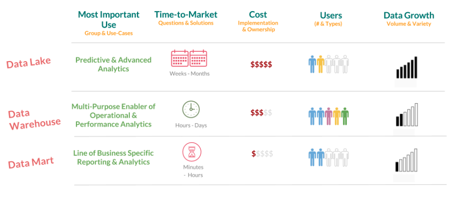Image credit Holistics.

Project Report

Objective - Heartrate Grade Resolution

Our specific objective is to create a data lake which includes extremely high resolution healthcare data tied to individuals. “Extremely high resolution,” is defined as body-process data down to the 1/300 Hz timestamp resolution.

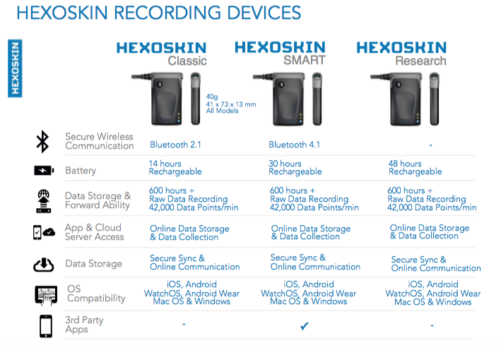
To collect this data, we used a product known as, “Hexoskin,” which captures ECG data through a bodysuit with sensors attached.

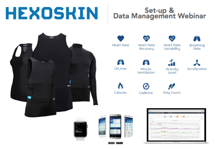
This suit has non-cloud based data capture devices which can capture and store localized highly detailed ECG data. Since Unix Time is typically limited to 0.01 second, and the storage requirement for ECG information is 0.003… the Hexoskin devices multiply Unix time by 256 in order to gain extremely high resolution for timestamps.

Using the above conversion, here is an example timestamp that Hexoskin would output for an ECG measurement:

Unix Time Milliseconds	Human Readable Time	Hexoskin Time
1498934654000	Saturday, July 1, 2017 6:44:14 PM	383727271424000

This type of resolution may be considered to be very high to be stored as individual json data points. Typical online audio streaming services today in 2017 measure at around 96kbps. Taking a typical json object example that we might extract and piece out, as shown below:

---

{
   "data":{
      "<datatype>":[
         [
            "383727271424000",
            "120",
            "10",
            "0.1",                        
         ]
      ]
   },
   "user":"9999999999"
}

---

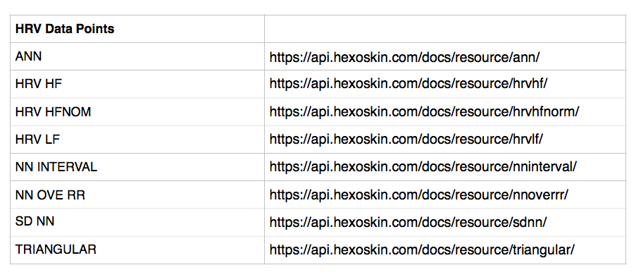
The first value is the Hexoskin timestamp, while subsequent values correspond to other either fundamental measurements at that time stamp or running calculated averages for other heart or lung measurements, with some examples shown here and below:

From the example above, we get a json object size of around 60bytes, which would translate to about 18kbps at that 300Hz resolution described above, meaning that at or around 96kbps is reasonable. Why would we need such high resolution, separated into individual data chunks? Basically, the science of the heart is very exacting, and there are micro-occurances which happen with each heart beat. To demonstrate, we can look at the typical heartrate QRS calculation:

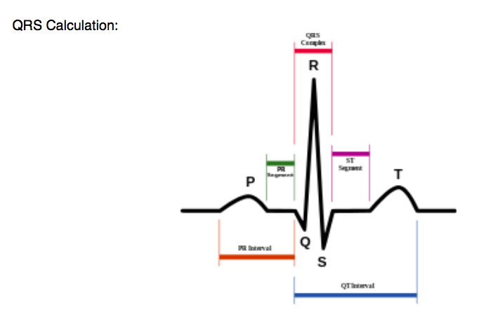
Basically, the QRS corresponds to three of the graphical deflections on an ECG chart, and is used to measure the balance between the left and right ventricle. Different types of QRS outputs can correspond to different conditions, and it is important to be able to measure the heart at a very high resolution to be able to capture the full QRS curve, which may happen within 80 milliseconds or even shorter at levels of high physical activity. The 1/300Hz resolution gives us ECG measurements at approximately every 3 milliseconds, which is a sufficient sampling frequency according to the Nyquist-Shannon sampling theorem, which shows that a function of maximum frequency \[B \] Hz, and sampling frequency \[f_{s} \] Hz, must follow the rule:

\[ B < f_{s} / 2 \]

Which, at 0.003… seconds heartbeat sampling rate, and 1/256 milliseconds underlying timestamp sampling rate, we are at an acceptable level for human heart measurements. A summary of what a single datapoint encompasses and how it is derived is shown below:

An example of some of the data captured during an experiment training with a local police force to determine stress levels under some standard training activities, we got the following chart, which I plotted in Matlab:

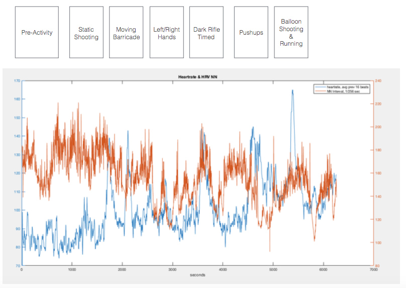
The blue chart shows heartbeat rate while the orangish red line shows continual Heart Rate Variability calculated measurements. This is significant because heart rate variability can be tied to stress and a predictor for post-traumatic stress syndrome as well as future heart attacks. So part of the reason why it would be interested to build a future, “ultra-healthcare-datalake” would be to be able to continuously monitor and store individuals’ heart rates throughout their lifetime, or perhaps at least in high-stress jobs and situations.

Previous Work On Abstracted Data Objects

ShareTrack is a previous hobby project I worked on which reported device-gathered data to the cloud. I gathered GPS data from various points of the world using a cellular GPS couple device, and reported the streaming data to an Amazon S3 Database. The data was all stored in a large S3 file which simply logged GeoJson objects sequentially, with the timestamp being recorded by AWS DynamoDB as the time of receipt of a given GeoJSON object. Each GeoJSON object looked like this:

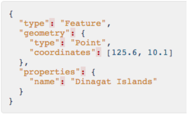
This format is standardized by a GeoJSON specification by the Internet Engineering Task Force (IETF), which makes it easy to decide as a format to use to create a type of base data object. If we were to turn this into our own personalized time-series data lake format, we might add a timestamp within that GeoJSON object, rather than relying on a pre-structured database time. Taking IoT considerations into play, the timestamp can be assumed to have been captured at the point of capture on the edge-device, rather than on the receipt at the server database, because the edge device is time synchronized with a cellular network, and would more accurately reflect the time and location of the physical object. We are making an important assumption here - that this way of formatting the data would give us a higher level of time-series precision to the data, assuming that our device is appropriately time-synced. In other words, devices should be authoring the time at which data is capturing, since they are doing the capturing, and embed that time within the data itself, rather than relying on the network effects of the data, which can be subject to unpredictable lags or losses of connection.

Real-Time Database Design Considerations

Databases are not magic devices but rather very complicated pieces of software in their own right. As discussed in this stackoverflow article, in general the database design is secondary to your business process design and should cleanly support your business [or organizational] process in a direct and simple way. That being said, before we fully jump in to building a data lake, let’s ask ourselves some general high-level database-design questions about the design, for sanity’s sake:

Question	Answer
Are you looking at a high-transaction rate, along the order of a busy website? Or are you looking at a small use case, on the order of a company HR system?	This depends upon the frequency of use of a particular device. Is this a weather station reporting the temperature once per day? Or is this a video or health monitor reporting on a patient 24-7?
Is security a big issue? Are you handling personal details, financial data or HIPPA data? Or is it just a product catalogue?	The larger the amount of data collected, the greater the security involved. The type of use case involved, health and financial record keeping being tied to the sensor data, will dictate the amount of security needed. For example, if the amount of corn sensed going through a silo over a huge number of silos is tied to the financials of a public company, this could be considered extremely sensitive data.
Will your users be doing any updates or inserts or is it read-only?	Typically in long-term IoT project, an, “update” would essentially be a report of a data point over time, while an, “insert” might refer to a new device being added to the system. These databases are very much read-write databases.
How many users, and what are the usage patters? Is there a peak load or is it evenly distributed?	Users of an IoT project could be considered as both the people reading the information generated and as the devices posting data themselves. Peak load in terms of reporting may be either consistent or concentrated based upon scheduling. Loading based upon reading depends upon the usage of the system.
Do you need 24x365 uptime? How much downtime for maintenance can be afforded?	Uptime may be constrained by the loading and reporting scheduling into the system.
How big is the database going to go?	This question is highly system dependent, but it is important to keep in mind that each individual device added is potentially creating a linear growth in the volume of data being reported - so database sizes can grow monumentally over time. With the pace of hardware and bandwidth development, and with the idea of different types of IoT data being reported into the same database, this linear function could become exponential. What’s important is to be able to calculate the size of a database may be over time.

How Time-Series Data Is Normally Stored

Database Type	Advantages	Disadvantage
Relational DBMS	Robust secondary index support, complex predicates, rich query language, etc.	Difficult to scale. Swapping in and out of memory is expensive. Tables are stored as a collection of fixed-size pages of data. Updating a random part of a data tree can involve significant disk I/O while reading from memory, and writing into a new system. RDBMS’s have challenges in handling huge data volumes of Terabytes & Peta bytes
Key-Value Store (Such as NoSQL)	Strong mathematical basis, declarative syntax, well-known language, using SQL. Basically, it runs well on cheap, commodity hardware. This architecture goes back to when Google had switched its datastore in the mid-2000s. Uses key-value pair type architecture, with a high throughput.	No strong schema of data being written/read. No real-time query management. No execution of complex queries involving join and group by clauses, no joining capabilities. Inconsistent transactions in terms of atomicity, consistency, isolation and durability. Not as, “high level.”

Convention says that time-series databases are typically stored in relational databases (table based) as opposed to NoSQL (document based) because they are cheaper, and ripe for holding huge amounts of data.

However, NoSQL and non-relational databases are the architecture which have been adapted in the age of Big Data. The thought is that for long-term database usage, they are more scalable. There are some contrarian points out there, but in general relational databases are designed for pre-defined processes, affordability and to have a rich relational interface between different datapoints, whereas non-relational is optimized for volume of data and putting the data scientist or discovery first. Healthcare, being an over $1 Trillion USD industry at this point, and having such a massive detrimental impact on society today and in the future with an increasingly aged population, is one of the most expensive data applications out there. Preventing or mitigating a particular type of condition for a person has a high monetary reward, with that monetary reward forecasted to go up in the ensuing decades, while at the same time the cost of data storage will go down in the ensuing decades, so we will for the purposes of designing for the future, assume a more expensive, flatter, lower time-decay data lake architecture.

Calculating Hypothetical Data Volume

We can make some brief assumptions by calculating the amount of data we may be inputing over a year using our current flatfile size discussed above. Of course this amount of data will increase by a certain factor when converted to a data lake format, but we can use this as a starting point.

Selecting from Existing Platforms

An exhaustive List of Various Types of Time Series Databases is provided by misfra.me.

Sampling of time-series databases geared toward IoT applications:

Database Name	IoT Specific Platform	License	Platform Built On	Database Model	Write JSON Protocol
InfluxDB	InfluxData	MIT		Relational Database	Uses line protocol for input rather than json.
	Cityzen Data				No information on website
	TempoIQ				No information on website
Atlas	MongoDB Atlas	GNU AGPL v3.0, Apache v.2.0	AWS	Document Store, Non-Relational	Individual Files or Documents
	Redis			key-Value Store
DynamoDB	AWS Dynamo DB		AWS	Document Store, Non-Relational

From the above analysis, we choose MongoDB Atlas.

Writing JSON Documents to MongoDB

• It is important to note that MongoDB formats JSON files on its end in a special binary format called BSON, which is essentially jSON with additional identification added.

Guide on Mongo Shell

We now know that we can connect to MongoDB, we can go in and actually start posting data. There’s a reference guide to go through with instructions on how to do that, but before we go that far, let’s take a look at how we’re going to architect our actual JSON documents. Architecting Our Data According to Standardized JSON Formatting

JSON vs XML

JSON documents are designed to contain data and be human readable. XML is designed to interface easier with web-based software. Both are human readable, but JSON is more modular for a variety of purposes.

The Input Datastreams

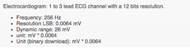
Each datastream from our origination / platform provider will come in a particular format. In our case, the data from Hexoskin can be accessed as flatfiles and CSV files, with each particular data type being described in the Hexostore API Documentation, also known as the, “Data Resources Document.” Each data resource has its own properties and specification about how it is stored and how to interpret the data once downloaded. For example, ECG data (electrocardiogram data) is documented here.

What we are seeing, when we receive ECG data, is voltage input data captured every 1/256 seconds (known as hexoseconds), at a resolution of 0.0064 volts per step. As we mentioned above in this article, the frequency is approximately 300Hz, derived from dividing unix time by 256.

• Note that, within the time domain, 1/256 hexoseconds is a regular number with a decimal value equal to 0.00390625 seconds.

Creating a Standard - Standardized JSON time series data (JTS)

The company eagle.io has published a standard for JTS, JSON Time Standard, with a tightly engineered specification for how this data structure should work. Though there is no IEEE or ISO standard for time series data at the time of this authoring, we can draw off of this existing platform’s standard to form our own specification.

Starting out, we are creating a simple data file, with one record per time stamp, and one time stamp per JSON object. So we will start out by populating the standardized data accordingly and manually, using an ECG record as a guide. We will create one JSON document representing the first measurement.

Timestamp

Each record contains an ISO8601 timestamp. Convert Postfix (Hexotime) to ISO8601 The first value in our timestamp is 384308888770, which is given in Hexotime, which is equal to (Postfix Time)*256.

To get the actual Postfix time, we divide by 256, which is equal to:

1501206596.7578125

Which in ISO8601 time is equal to: (measured in UTC)

2017-07-28T01:49:56.757Z

Note, the smallest fraction of time that ISO8601 as specified by the above data structure is shown to be equal to:

0.001 seconds

To test, the next time value up on our database is equal to 384308888771, which coverts to:

2017-07-28T01:49:56.76Z

Which is precisely 0.003 seconds greater than the previous timestamp, fitting within our resolution. This level of precision works for differentiating between 1/256 seconds at Hexoseconds (which is equal to 0.00390625 seconds per Hexosecond), but in order to achieve another Hexotime variation at 1/4096, we would need a higher resolution at:

0.000244140625 seconds per hexoseconds_4096, therefore 0.0001 seconds

We will also need to be able to convert our time down to the faction of the second necessary in order to process hexoseconds_4096. That being said, the actual technical documentation for ISO8601 says that there is no limit to the number of fractions of a second that can be used to express a particular point in time, as long as it is understood by both communicating parties what the maximum resolution used will be. Moving on to the actual data reported in the JSON file, we have header columns:

id	For the ID, we can use the id of the actual device which recorded the data in question, or the record origination from where the originally came. Since the metadata of a given device or part number is not included anywhere in the metadata, we will default to the record id.
name	This, quite obviously will be used to designate the name of the sensing resource, e.g. whether it be ecg or acc, etc.
dataType	This will set the actual datatype itself, the types of which can be found in the table below. For our purposes this will be set to, “NUMBER.”
renderType	This will let the render type of the ‘v’ attribute in the data record below. The renderType can either be, ‘STATE’ for string format or ‘VALUE’ for number format.
format	Specify how the value should be formatted for display. Number Parameters use this setting to set how many decimal places should be shown (leave empty to display the value with all included decimal places). 0 will always display a digit. # will only display a digit if it exists. Time Parameters use this setting to determine the formatting of the timestamp (leave empty to display timestamps in your default user time format). Select a preset format from the drop down list or specify a custom format using time format tokens.
aggregate	Default is NONE.

Once we have our standardized base data format created, we can then import data into our selected database platform, MongoDB.

Importing into MongoDB.

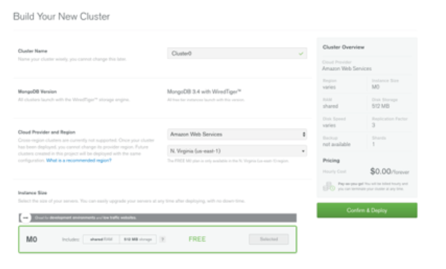
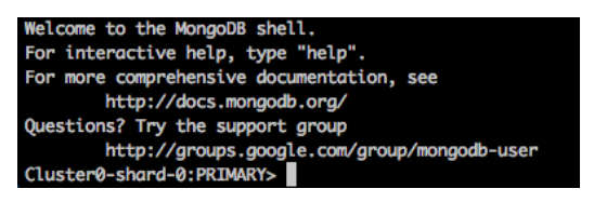
To start off with, initialize a MongoDB cluster.

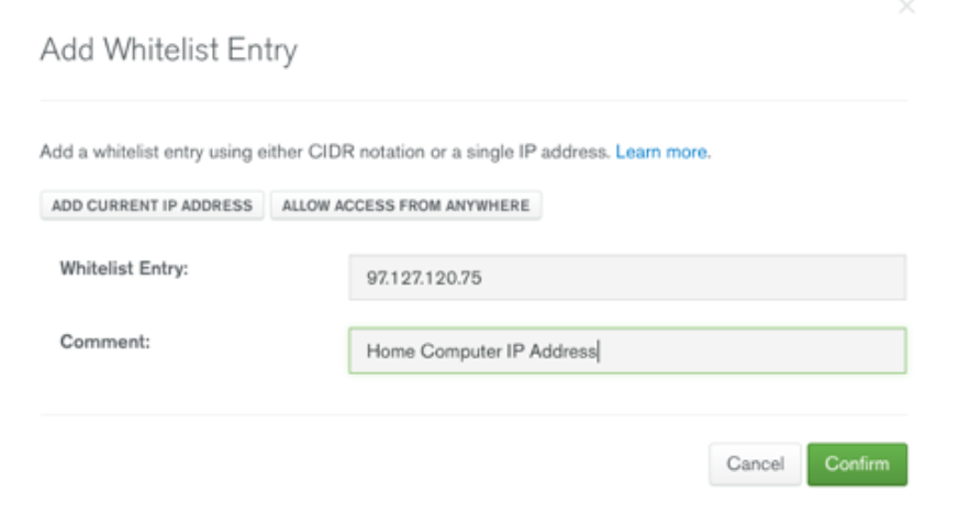
Then, whitelist an entry point to that cluster - in our case we were just using a local computer.

Then, connect to the cluster.

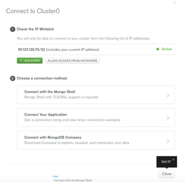
Once connected, you can use the MongoDB CLI to connect to the MongoDB shell.

Our accepted time stamp will be the same as the beginning and end record for this particular point. Thus, for ECG our final test data point, representing the first collected datapoint as a sample will look like the following, which is based upon a modified version of the eagle.io timestamp standard mentioned above:

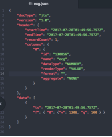
Looking at the output size of this document, we can see that it is 598 bytes.

For two hours worth of data at this 1/256 hexotime recording factor, we will have 1,457,152 JSON documents, amounting to:

(1,457,152 timestamps)*598 = 871,376,896 bytes = 871.37 MB worth of data.

Whereas the originating flat file from Hexoskin included 26.2MB of data. This represents an increase factor of 33.2X. It’s possible that we could re-engineer this JSON file from a fundamental level and come up with a much lower-memory requirement specification, but for now we will keep it as is.

Now that we have one finalized JSON document we can experiment with populating it into MongoDB. Various transforms in Python or a specified chosen language can be used to transform and rip the data from its raw, original format and populate it into MongDB.

Analyzing Pricing

MongoDB sells its structure by cluster on either on-premise computing services or based upon a chosen service provider, AWS, Azure or others. There is a multi-region version for advanced accessibility.

If we imagine a non-regionzlied version of the database which spits out data and insights along with a lag time in the several tens of microseconds to five microseconds being acceptable for report generation, we can assume non-regionality as being acceptable.

Part of the pricing consideration is of course the input and output disk memory necessary to utilize the database. As an abstraction, a database is not simply a table or collection of data, there is also computing power, e.g. a processor memory, needed to extract and input data from a given database cluster.

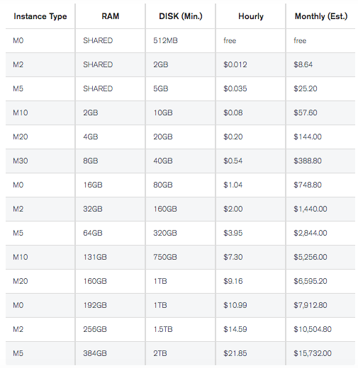
Looking at an example, we can see MongoDB’s offering of their service on top of AWS.

In addition to the overall storage and usage fees, there are also data transfer fees, which are fairly negligible:

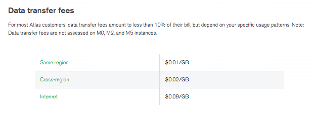
So let’s say we were capturing data for a high-risk profession 8 hours per day, 5 days per week, 40 weeks per year. How much data would we aggregate over a year timeframe? Assuming 800MB of data every two hours:

(800MB)*(4)*5*40 = 640,000MB = 640GB = 0.64TB Per Year

Using the low processor power version of the AWS deployment, this would work out to about $48,470 worth of server time per person per year at current pricing. This sounds incredibly expensive, however, keep in mind the cost of storage memory over time has decreased relatively logarithmically:

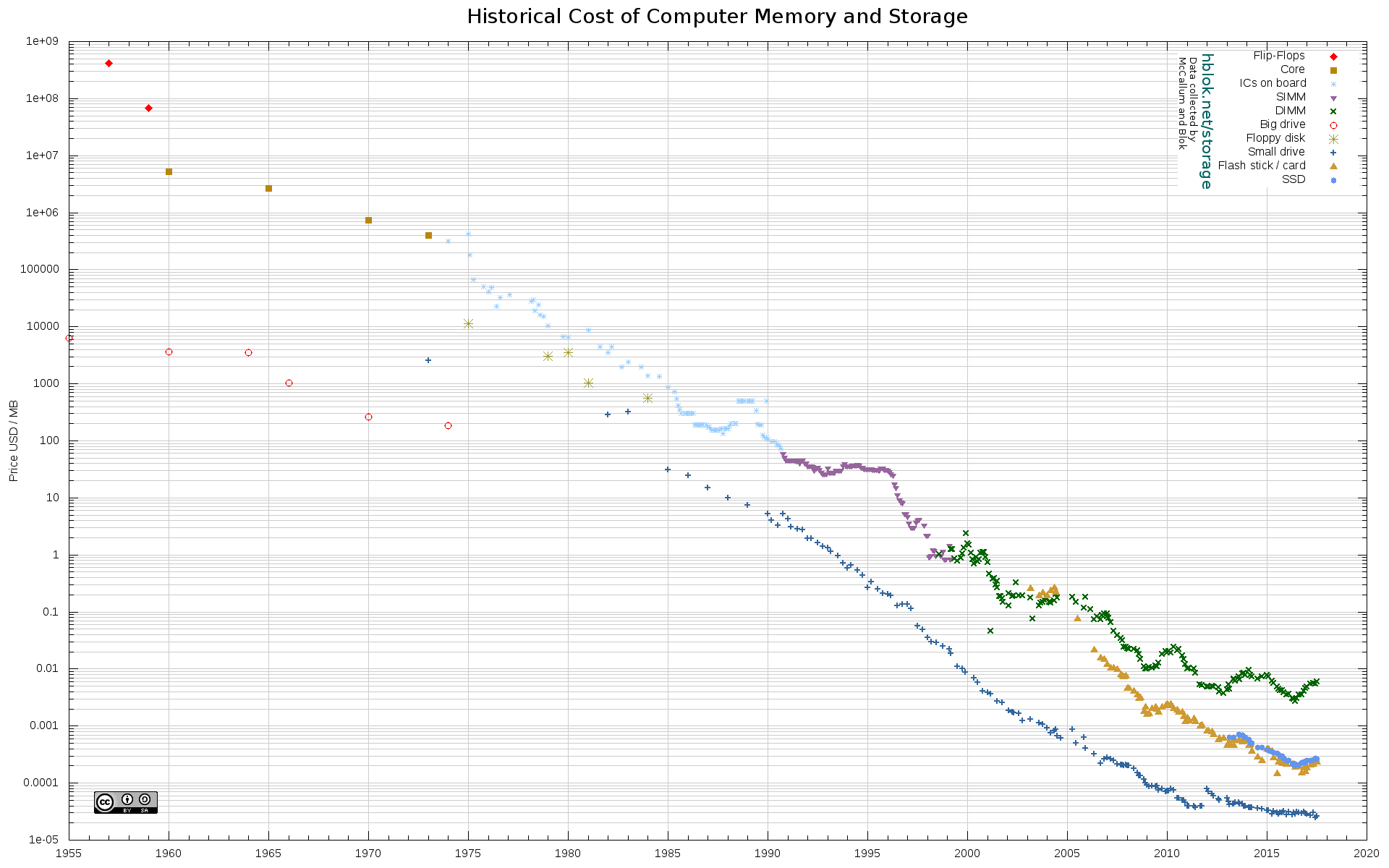
So, it is reasonable to believe that in a decade, the costs could go down by almost an order of magnitude, or perhaps within the range of effectively $4000 per year, and the decade beyond that, closer to $400 per year, or $30/month.

This of course ignores any cost efficiencies which may be built in by transforming older data into larger and slower access file sizes, and later, “pulling and querying,” those access file sizes into cheaper storage formats.

Beyond this, just storing raw datatypes in an actual cloud service provider system such as Azure, while more labor intensive on the setup side than an already built application such as MongoDB, already provides the relatively $30/month pricing at our suggested usage levels above. If there is a clear business model for an, “ultra-healthcare-data-lake,” with funding behind it, it may make sense to build that out, spending on the front end and use raw cloud services to lower the cost per user right out of the gate.

Conclusion

Why Not Keep Everything as a CSV or Flat File? If data lakes are so expensive, why not just avoid them all together for cost purposes? In Summary:

The lifetime value of the data in the form of individually accessible pieces is more important than the optimization of the actual data itself.

Healthcare and indeed other industries and sectors are ripe for either saving money through efficiencies, identifying larger risks and underwriting and future threats, or even selling additional services based upon currently collected information. Rather than dismissing data lake approaches and hand-waving them as, “too expensive,” it is important to take an actual look at the costs through various providers and solutions to be able to determine whether they work for a given problem set, as the payoff can be massive when considering the insights derived from the data rather than just the cost savings of how the data may be stored.

As the amount of data we generate and consume continues to go up exponentially in sectors ranging from healthcare internet of things to industrial, agricultural or other industries - it is important to have a general feel for what applications cost what amount, to be able to communicate to non-technical team members.

Roughly what we found here is:

• For measuring a super detailed picture of someone’s heartbeat on the job most of the year, such that it can be queried by data scientists, that costs roughly $3000 per month today for an, “already built service,” and roughly $30/month for a service which requires some leg work to get going.
• That same application will probably cost roughly $300 to $3 per month 10 years from now, and $30 to $0.30 per month twenty years from now.

Plan accordingly!

Check out my Portfolio

Data Engineering, Healthcare, Internet of Things, Machine Learning

Share